• Schematic (native Eagle format)
• Schematic (JPEG)
• Layout (JPEG)
• Spice simulation circuit (native 5Spice format)
• Spice simulation analysis (5Spice)
• All files

NOTICE: This webpage and associated files is provided for reference only.  This is not a kit site!  It is a collection of my work here at the University of Toronto in the Physics department. If you are considering using any schematics, designs, or anything else from here then be warned that you had better know something of what you are about to do.  No design is guaranteed in any way, including workable schematic, board layout, HDL code, embedded software, user software, component selection, documentation, webpages, or anything.

All that said, if it says here it works then for me it worked. To make the project work may have involved undocumented additions, changes, deletions, tweaks, tunings, alterations, modifications, adjustments, waving of a wand while wearing a pointy black hat, appeals to electron deities and just plain doing whatever it takes to make the project work.

The pulse laser under test produces a series of optical pulses, part of which is directed to a photodetector that generates an electrical pulse train.  The pulses are Gaussian of around  50-100mV peak, about 1.5-2nS width, pulse repetition rate 7.5nS, total train duration ~100 pulses up to max around 6-10 µs.  Although no single pulse has to be measured, periodic measurements are taken throughout the pulse train.  By integrating the area under the pulses and knowing the envelope shape, the amplitude of  groups of pulses can be extraoplated.  This circuit does the integration.

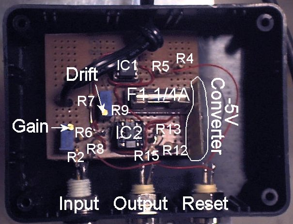
Connection and Operation

Connect the photodiode/TIA to the Input, connect a 'scope or ADC ("Analog to Digital Converter") to the Output and connect a TTL control to the Reset input.  With Reset at logic "0" (low), the Output integrates the input.  With no signal input, this integration can be positive or negative depending on offsets and errors - see the Static Calibration section below. Operation is a three-step process: a drift calibration, the measurement run and and a second drift calibration.
To measure a pulse train, leave Reset active (high) until >>10uS before the pulse train starts.  Continiously measure the Output before, during and after the measurement run.  In the 10uS immediately before the measurement run when there is no signal, measure the Output's drift.  Note the start and end voltage during the measurement run.  In the 10uS immediately after the measurement run when there is no signal, measure the Output's drift again. Subtract the average of the two drift measurements from the actual measurement run to obtain the true integral of the pulse inputs. The Reset may be asserted high at any time before the next run.  The Output has an active range of ±4.5V, Output saturation is harmless.  The Input is designed for low level pulses as described above but is reasonably accurate on significantly smaller, larger and longer pulses.  Bandwidth is estimated at 10GHz for -3dB, rolloff is deterministic and repeatable so can also be compensated for.  Note that the drift may be negligible and if so, ignored.
A gain control is provided to adjust the slope of the integration.  Adjust for an Output of several volts by the end of the measurement run.

Static Calibration

Modus Operandi

The problem with integrating pulses in the GHz region is that no classical opamp integrator will respond fast enough, or at best will roll off harmonics.  Properly selected passive R and C components can have wide bandwidths.  A simple RC integrator (AKA low pass filter) will work only if the length of the pulse train is much shorter than the RC time constant.  Too short a time constant and the RC just averages the amplitude.  Too long a time constant means better integration but also lowers the sensitivity to below the noise threshold.  In other words, the very beginning of a logrithmic rise to a limit is virtually linear.
Looking at a single pulse into an RC integrator, a single positive pulse will put a small charge into the capacitor C1, appearing as a voltage given by the linear charge equation V = I*t/C, where the charge current I is Vpulse / R.  Immediately after the pulse, there will be a small positive voltage across the resistor R1.  It will dissipate by the RC time constant. However, using R3 and C2, U1 integrates this unwanted residual voltage.  U1 will continue to relatively slowly integrate any voltage across R1.  The circuit's output voltage is taken from the integrator U1 output.
A voltage feedback opamp was selected with high GBW to track the R1*C1 time constant as fast as possible, however a high slew rate is not needed.  By juggling the R1*C1 time constant against the R3 & C2 integrator timing, the integrator bandwidth is at least an order of magnitude faster than what the opamp alone would be capable of.  The integrator is sensitive to Vio so it has to be trimmed out out with either a trimpot or DAC.  An analog switch resets the integrator for the next pulse train.

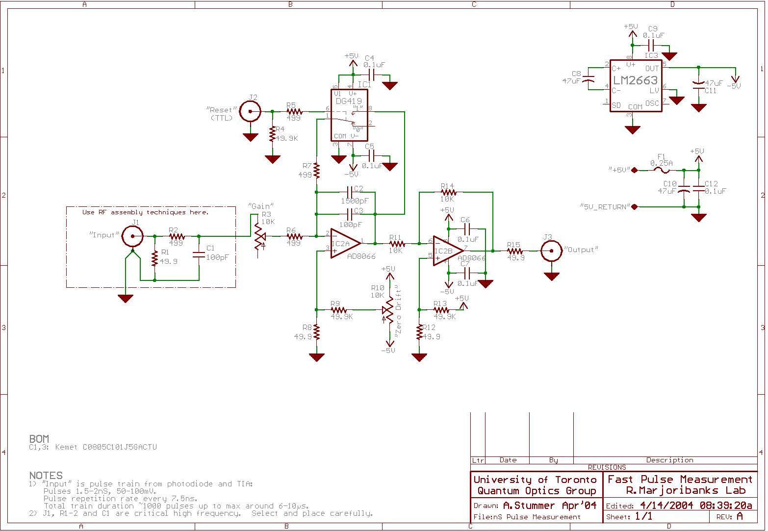
The circuit was drawn in Eagle and simulated in 5 Spice. All schematics, simulations, associated files and pictures are in the directory.