Femtosecond Fiber Laser Behaviour

Stable modelocked pulsetrain

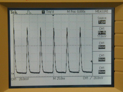
A good modelocked pulsetrain will appear as at right, on a Tektronix TDS210 oscilloscope. Do not forget to turn on the InGaAs photodetector, which has a battery inside to provide a bias voltage. Do not forget to turn it off, when you leave the lab.

This scope has a bandwidth of only 60 MHz, not enough to resolve any details of the pulses, except when gross multiple pulses are created. Oscilloscopes used for laser work are usually at least 400 MHz, and increasingly better than that.

Stable modelocked spectrum

A good modelocked pulsetrain will produce a spectrum as at right on the Ando Optical Spectrum Analyzer (OSA). The OSA can be controlled from front-panel buttons, but can also (and sometimes more easily) be controlled over GPIB from the LabVIEW program "AndoOSA.vi" This also permits saving datafiles in spreadsheet format. You should not use the thermal-paper printer built into the OSA: it's an unneccessary expense, and the printout fades in room light over a matter of weeks.

The spectrum at right has a bandwidth of about 35 nm, which is sufficient to support pulses of 100 fs, if there is no frequency chirp or other phase distortion on the pulses.

Unstable behaviour

Many interesting things can happen with the laser, and this sort of laser behaviour is the subject of current academic research.

The changing pulsetrain at left is accompanied by the changing spectrum at right. You can see as secondary pulses evolve and drift in time across a background of a regular pulsetrain. A whole universe of nonlinear behaviour, including the appearance of solitons, and soliton-regime operation of the fiber laser for pulse-formation/modelocking.

You are welcome to play with this behaviour, to discover what settings produce different sorts of behaviour. There is a close connection between the time-domain signal from the oscilloscope and the power spectrum that accompanies it, although neither shows exactly the electric field in time or frequency domain, E(t) or E(w), which are Fourier transforms of each other. Basically, two pulses spaced by a time separation will interfere in frequency-space to make the fringes you see in the spectrum; the fringe spacing is = 1/.

Investigating this behaviour is part of one of the advanced sections of this lab.

Polarization controlle

Last revised: 16 March 2003 - rsm