Several bits of interactive software have been developed to help you manipulate parameters of -- to play with -- the optical physics concepts and the laboratory tools used in this laboratory. These should all be available in the Fiber Laser Experiment folder on the laboratory PC dedicated to the Femtosecond Fiber Laser experiments.
Kaleidagraph™, from .Synergy Software, is installed on lab machines. A free trial is available online, which will not let you save, but which will let you work on a home machine and copy and paste a graphic of your results into a formal report or writeup.
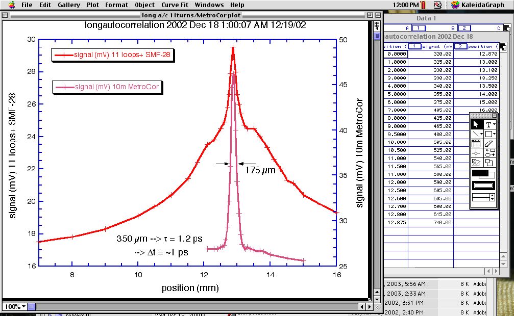
The software is quite powerful, and supports curve fitting from a large family of types, and from function definitions you make yourself. It can be useful in fitting spectra or autocorrelation traces, and finding the FWHM of such profiles. It can also make nice plots from data acquired from the beam-profile webcams, using NIH Image or Scion Image to make a lineout profile, saved as a file of data points.
A quick-start guide may be quite helpful to you, in getting started with Kaleidagraph.
![]()
StarOffice™ is available on lab machines; it is a Sun Systems product now sold at modest cost (~ CAD $100) with roots in open-source concept freeware; an OpenOffice version is available free online from the same site.
The software is powerful word-processing, spreadsheet and presentation software which is quite compatible with Microsoft Office™ software.
![]()
Oscilloscope, autocorrelator and OSA files take up quite a lot of space: a USB-2-wired CD-R/RW burner is available for you to preserve your work, to keep a copy for putting results into a formal report, or to take results home for further analysis.
You may have to put your student card on deposit in the Equipment Room in exhange for the burner, or it may be available on the beam-profiling computer. Note that only certain ports on the computers may be USB-2, needed for high data throughputs.
![]()
 (interactive illustration
software)
(interactive illustration
software)You're likely familiar with linearly polarized light, and probably with circularly polarized light; possibly you've been introduced also to the more general case, elliptically polarized light.
Elliptically polarized light is necessary for mode locking, in the fiber laser, and the Primer describes how the polarization controllers use oriented stress in the glass to alter polarization states. The Primer also describes how nonlinear effects of intensity cause rotation of the ellipse axes (Kerr elllipse rotation); this is illustrated in an animation lower in this page.
All the examples of elliptical polarization are equivalent to simple Lissajous figures (if you know of this from Waves and Vibrations), ones which have the same frequency of drive on both the x- and the y-axes. Changing the amplitude and relative phase changes the size and orientation of the ellipse produced.
This demo program lets you alter the amplitude, and the relative phase, while animating the result. It should help you get a feel for elliptical polarization states, and how they're manipulated in our fiber laser.
Much as is introduced in the acoustic waveguide experiment, the boundary conditions of a waveguide structure -- including an optical fiber -- make certain impositions about what frequencies can propagate, and what effective wavenumber they'll have as they move down the structure. Whenever these are not proportional, as they are for light in vacuum and usually for sound in free space in most gases, the wave is dispersive.
As described in the Primer for dispersion, provided in the acoustic waveguide experiment, this means that the energy associated with different frequencies will propagate at different speeds, i.e., that the group velocity is frequency-dependent. Consequently, the pulse will unravel or unspool with time, as this animation at right illustrates.
Dispersion results not only from the boundary conditions of a waveguide structure (modal dispersion) but also from non-constant index of refraction in materials, for different wavelengths (material dispersion). A glass fiber has both, and by changing the type or impurity-doping of the glass, or by changing the transverse dimension of the core of the fiber, quite different dispersion characteristics can result. Nanostructured materials, like photonic bandgap fibers (holey fibers) have repeated boundary conditions, and can have enormously strong dispersion effects, which can be adjusted or tuned at the design stage, or sometimes even in use.
In the Femtosecond Fiber Laser experiments, you can show how different optical fibers have different values of dispersion, measuring with the autocorrelator the duration of pulses chirped in different lengths of different fibers. You can also show that even the sign of dispersion may be different in different types of fibers, so that you may stretch a pulse out in one optical fiber, and then put it back together with another.
In an advanced experiment, you can see that amplification of a pulse also produces dispersion, and you can measure the amount of dispersion resulting from different gain-factors. Finally, you can show that a pulse which has been stretched by such amplification can be compressed again, using the right length of the right kind of fiber.
This animation shows a pulse with an initial frequency chirp as it is compressed by suitable dispersion in a medium or fiber. The blue line shows the evolving pulse duration; the green line shows the evolving pulse intensity. Some nonlinear effects come about only near the peak compressed intensity.
The fiber laser Primer describes how Kerr ellipse rotation works: basically it is an intensity-dependent precession of the major/minor axes of elliptically polarized light, as illustrated by the animation at right.
Most simply, it comes about because intense light alters the index of refraction. Along the major axis of the ellipse, the light sees a higher index than along the minor axis of the ellipse. So, there's a birefringence that changes the phase slightly between the electric-field components along the major and minor axes. In small amounts, such birefringence looks like a slight rotation of the ellipse. As the ellipse rotates, though, the induced birefringence necessarily follows the ellipse around, so there's an incremental but continuous change in orientation.
Why does this matter? It's this rotation, initially only of the most intense random fragments of light, that brings about the formation of short pulses. In a 'survival of the fittest' scenario, the polarization controllers are adjusted to prepare and then receive elliptically polarized light in a particular way -- light which rotates its ellipse the right amount is optimally converted to linearly polarized light and survives the polarizer (built into the isolator). Light which is too weak (or, for that matter, too intense) suffers greater loss of energy, dumped by the polarizer.
Thus, even the more-intense 'middle' of a pulse survives better than the lower-intensity wings, and sees more net amplification. Thus any pulse will peak up in the middle, or have the wings suppressed, which decreases the FWHM. Repeated many times, for each of many round trips, the cumulative effect is quite pronounced, and 100fs pulses can easily result.
![]()
 (interactive
illustration software)
(interactive
illustration software)This software helps you develop an instinctive understanding of the autocorrelation traces you will produce, especially with the long-baseline (picosecond) configuration.
You can put in transform-limited or linearly chirped pulses, examine the spectrum expected, see the effect on the autocorrelation of pulse duration, dispersion, gaussian vs. sech^2 pulses, an autocorrelator that has two arms not quite balanced in intensity, and the effect of having two pulses in the output, spaced too closely to be detectable by the oscilloscope and fast photodiode detector..
The software permits you to save the output datafiles for the pulse generated, its spectrum, and the autocorrelation as well. Saved as tab-delimited spreadsheet files, they may be imported directly into Kaleidagraph or Excel, both of which are on the lab computers.
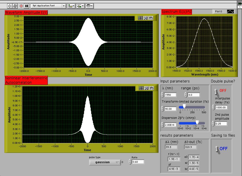
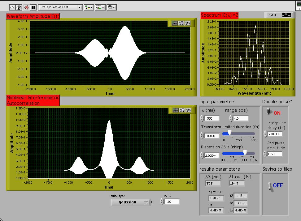
Left: 100fs pulse stretched to ~300fs; Right: 2 100fs pulses separated by 750fs
(click on either image, to enlarge)![]()
This instrument can be controlled by the PC dedicated to this experiment, by a LabVIEW virtual instrument, communicating over a GPIB bus. This will permit setting the parameters for wavelength, resolution,
To use the ANDO OSA by computer:
You can learn more about the principles of OSAs from the book by Derrikson, available at the 2nd floor labs equipment office.
You can learn more details about the ANDO AQ-6310C Optical
Spectrum Analyzer from the technical
manual (4.1 MB), though it is not at all a good place to learn
the basics.![]()
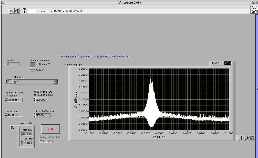
The Tektronix TDS210 oscilloscopes in this lab can be controlled by the PC dedicated to this experiment, by a LabVIEW virtual instrument (VI), communicating over a GPIB bus. The VI is a very close 'clone' of the front of the scope, and all of its functions, and is nearly self-explanatory. In addition, though, it permits you transfer and save to a spreadsheet file the waveform you record. This tab-delimited file can be imported directly into Kaleidagraph or Excel for analysis, plotting, or inclusion in your written reports.
The Tektronix TDS210 oscilloscopes in this lab can be controlled by the PC dedicated to this experiment, by a LabVIEW virtual instrument (VI), communicating over a GPIB bus. The VI is a very close 'clone' of the front of the scope, and all of its functions, and is nearly self-explanatory. In addition, though, it permits you transfer and save to a spreadsheet file the waveform you record. This tab-delimited file can be imported directly into Kaleidagraph or Excel for analysis, plotting, or inclusion in your written reports.
You can learn more details about the TDS210 digital oscilloscope
from the Instruments
and Tools page. You can also learn
about using oscilloscopes, or get more specific
information and specs for the TDS210. ![]()
Last revised: 6 April 2003 - rsm