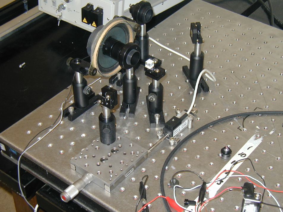
This is a Michelson interferometer with one arm mounted on a translation stage, used to make both arms of the interferometer of equal length. The second arm uses a corner-cube retroreflector mounted on an audio speaker -- even if it wiggles, it sends the beam back as it came in. The audio speaker is driven by a sine wave from a function generator: as it oscillates, it scans one 'copy' of the pulse through the other copy, as they propagate together to the detector. The oscilloscope is triggered by the function generator, so the oscilloscope shows a repeatable scan, with time proportional to relative displacement of pulses in the autocorrelator.
![]()
This is the simplest configuration of the autocorrelator: a speaker moves the corner-cube mirror, to scan path differences in the two arms by about 0.5 mm. This is suitable for use with pulses up to about 2ps duration.
Setting up the autocorrelator, if someone puts it a long way out of alignment, is easy for an experienced person, but you may want some help when you first try it. Unless someone has sat down on the autocorrelator, only minor alignment of the 2nd arm's flat mirror onto the detector will be needed.
- use the oscilloscope with AUTO trigger, and a fast timebase of about 10 µs/division to see the signal from the photodiode during initial adjustments
- connect the two 9V batteries to the amplified photodiode
- use the IR card and dim room-lighting to see where the beams travel
- put the beam through the middle of the beam-splitter, and travelling quite level through to the flat mirror (use a ruler, and tape the card to it)
- the beam should be level also to the corner-cube retroreflector; it should hit the dead centre of the corner cube -- this is important in getting good fringes later
- the beam should hit the centre of the lens -- if it does not,, and there is no signal whatsoever from either arm, you may have to reposition the detector. For that, you may have to remove the black infrared-pass filter to see the lens
- set the micrometer on the translation stage to the position for the two arms to be the same length (in March 2003, this was a setting of 12.45mm)
- run the waveform generator to drive the speaker with a range of about 1 mm
- block the arm with the flat mirror, so you see only the signal from the retroreflector, which cannot be adjusted
- run the oscilloscope on auto-trigger and a 1 ms or faster timebase
- using a small Allen key to make fine adjustments to the 45° flat mirror, maximize the signal on the oscilloscope (~50 mV is good)
- unblock the flat-mirror arm, and use the IR card and dim room-lighting to see that the two beams overlap; use the small Allen key to adjust the end mirror in that arm to bring the two to overlap on the card
- block the corner-cube arm, and again make fine adjustments to maximize the signal, this time from the second arm
- put the oscilloscope time-base on 10 ms/div, and trigger it from the synch (TTL) pulse of the generator
- unblock both arms; you may immediately see signal with fringes, or you may have to make very fine (less than 1/16th of a rotation) adjustments of the mirror in the second arm until you do
- if the multiple signals you see (from corner cube inward, turning and going outward) are not evenly spaced, adjust the translation stage micrometer slightly (less than 100 µm) so that the laser pulse hits the corner cube as it passes the middle of its oscillation range. You may have to touch up the alignment again.
A nice feature of the interferometric autocorrelator is that the fringes calibrate the device for you!
To interpret the signal you see, you may want to try the demonstration Autocorrelation Illustration. In that, you can set the transform-limited pulsewidth, and also the chirp, and see the autocorrelation patterns produced. It's the fastest way to understand what you are seeing.
![]()
For longer pulse durations, or to look at multiple pulses separated by up to about 25 ps, you can hold the speaker-mirror still, and move the other mirror through a much longer range. In that case, a LabVIEW program records the position of the translation stage, and the signal from the Si photodiode detector, provides excellent filtering of the signal, and plots it for you. It also give you the chance to save your data in spreadsheet format.
- first get the autocorrelator working nicely in moving-mirror mode, above. This is easiest using a short pulse from the fiber laser using the ~2m orange (MetroCor) fiber provided, and the laser operating in its most basic modelocked mode.
- stabilize the speaker: unscrewing the black 1" diameter 'lens tube' in it's adjustable mount, make it touch the aluminum base which holds the corner cube on the speaker-cone. About 500 µm after touching the aluminum should be enough. This will make the translation stage the only moving element.
- rebalance the arms: put the oscilloscope in AUTO trigger, and the timebase about 25ms/div. Since you moved the speaker slightly, you need to move the translation stage the same way to compensate, keeping the paths about equal length and the signal near the peak of the fringes. As you twist the micrometer, you'll see that you run through all the fringes, on the oscilloscope. Once you see clear evidence for the interferometeric part, just guess where the most intense is, and that will be fine!
- attach the 9V battery for the position sensor circuit
- null out the position-sensor signal: a blue plastic potentiometer lets you set the bias voltage for the position sensor, once the arms have been rebalanced above. Using a voltmeter, set the signal from the BNC cable attached to the position transducer to a magnitude smaller than 10mV (the point of this is to simplify the way that voltages are accurately digitized)
- connect the position sensor BNC to channel ACH0 on the data acquisition box (NI DAQPad6020)
- connect the photodiode output BNC to channel ACH1 on the DAQPad6020. Power the DAQPad ON
- launch the long-timebase autocorrelation controller LabVIEW VI
- move the translation-stage position to off-balance the interferometer by a few mm
- click the RUN button on the controller VI, and immediately begin scanning the translation stage back over the balanced-arm position and beyond. The software will run for a few seconds (adjustable), and then display the autocorrelation over the range you've made
The fringes can alibrate the device for you, as above, or you can figure out the relationship between mV in the position sensor and mm on the translation stage, and convert accordingly using the speed of light (and double-passing the arm with the translation stage).
To interpret the signal you see, you may want to try the demonstration Autocorrelation Illustration. In that, you can set the transform-limited pulsewidth, and also the chirp, and see the autocorrelation patterns produced.
![]()
Last revised: 6 April 2003 - rsm