Faraday Tutorial 1
Jason Harlow
Task: Make a plot of the voltage versus
current data for a 200 Ω resistor, and fit a straight line. Compute χ2 for the fit. Also, explore higher order fits and fix the “Use
Significant Figures” option.
Imagine you have a circuit which contains a 200 Ω resistor, and you want to confirm Ohm’s Law by measuring current and voltage. You set up a DC voltage across the resistor which you vary from 0.1 to 20 mV. You set up an ammeter which reads the current through the resistor at all of these voltage settings. Your data are:
|
V (mV) |
V error (mV) |
I (μA) |
I error (μA) |
|
0.1 |
0.05 |
0.39 |
0.05 |
|
0.5 |
0.05 |
2.59 |
0.05 |
|
1 |
0.05 |
5.04 |
0.05 |
|
1.5 |
0.05 |
7.4 |
0.05 |
|
2 |
0.05 |
9.7 |
0.05 |
|
4 |
0.05 |
20.52 |
0.1 |
|
6 |
0.05 |
30 |
0.1 |
|
8 |
0.05 |
41.55 |
0.2 |
|
10 |
0.05 |
51.07 |
0.5 |
|
12 |
0.05 |
62.9 |
1 |
|
14 |
0.05 |
66.5 |
2 |
|
16 |
0.05 |
78 |
2.5 |
|
18 |
0.05 |
91 |
3 |
|
20 |
0.05 |
98 |
3 |
1. Make a data file. Save the data in a text file, r200ohm.txt, with tab-delineated columns. That means that each line of the text file has four entries, and after each entry there is a “TAB”. The file must contain columns of numbers only, with no headings on the columns. Many data taking programs, such as Labview, output this type of file, and you can import it quite easily into a spreadsheet. You can download the data here: r200ohmj.txt
2. Start the Faraday fitting program. Open a browser such as Firefox or Internet Explorer and go to http://faraday.physics.utoronto.ca . Click on Data to go to Data Analysis Tools. Click on Linear Fit and enter your faraday login and password. If you do not know these, you can ask the Advanced Laboratory Coordinator.
3. Upload your data into Faraday. Click on “from the filesystem on your computer”. Leave the line beside “Variable names (optional)” blank. By the line beside “Data Values:” click on Browse. Click on r200ohmj.txt, which should be sitting in one of your directories. Click on Open. Click on Submit Upload.
4. Select the variables for the fit. Since there are four columns in the data file you uploaded, the program should recognize four variables, which it automatically calls var1, var2, var3 and var4. In your case, these refer to voltage, voltage error, current, and current error, respectively. In this experiment, voltage was selected by turning a knob, so we call it the “independent variable”. The resulting current for a given voltage was measured, so we call it the “dependent variable” (because current depends on voltage, in this case).
· Beside Dependent variable click var3 .
· Beside Error in the dependent variable click var4 .
· Beside Independent variable click var1 .
· Beside Error in the independent variable click var2 .
5. Select the powers for the fit. You can fit up to a ninth order polynomial of
the form ![]() . Check the boxes
corresponding to the parameters Ai
that you wish to fit. These parameters
will be adjusted to minimize χ2. Any boxes you do not check
will force Ai=0. If you want to do a linear fit, put a
check-mark in “0” for y-intercept and “1” for slope. Or, since the current should in theory drop
to zero when the voltage is zero, you can choose to force the y-intercept to be
zero by checking only the “1” box. This
is preferable since it reduces the number of degrees of freedom of the fit.
. Check the boxes
corresponding to the parameters Ai
that you wish to fit. These parameters
will be adjusted to minimize χ2. Any boxes you do not check
will force Ai=0. If you want to do a linear fit, put a
check-mark in “0” for y-intercept and “1” for slope. Or, since the current should in theory drop
to zero when the voltage is zero, you can choose to force the y-intercept to be
zero by checking only the “1” box. This
is preferable since it reduces the number of degrees of freedom of the fit.
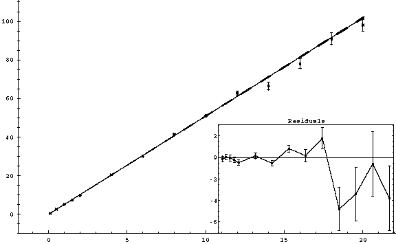
6. Perform the fit. If you followed the directions above exactly with a fit with A0=0, you should end up with a plot like the one below.

the slope
is 5.09 ± 0.022 micro-Amps per milliVolt,
corresponding to a resistance of 196.46 ± 0.85 Ohms. The χ2 is 27.63 for 13
degrees of freedom, which represents a fairly good fit. Generally, χ2 should be
between about 0.5 and 2 times the number of degrees of freedom. A low value of χ2 means the
fit it “too good”, usually indicating that your error bars are either
overestimated or not representative of the scatter in the measurements. A high value of χ2 means the
points are on average further from the fit than they should be, given the
errors. This usually means there is
something wrong with your theory or measurements.
At this point you can print the fit if you wish. There are ways to add labels to the fit which I will not detail in this tutorial. Here is a warning: when performing higher order fits, you may wish to turn off the “Use Significant Figures” option, which is on by default. This has confused many students in the past, so I will give an example.
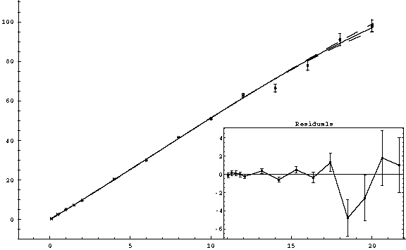
Suppose we wish to perform a higher order fit on r200ohmj.txt, even though we know that the current versus voltage should be linear. If we choose to fit A0, A1, A2, A3 and A4, (4th order polynomial) we get:

A slightly curved line with a χ2 of 19.14. The residuals are similar or slightly less than they were for the A1 only fit. It make sense that as we add more parameters, the curve more closely tracks the data points, and the residuals decrease. However, if we choose to fit A0, A1, A2, A3, A4, A5 and A6, (6th order polynomial) we get:

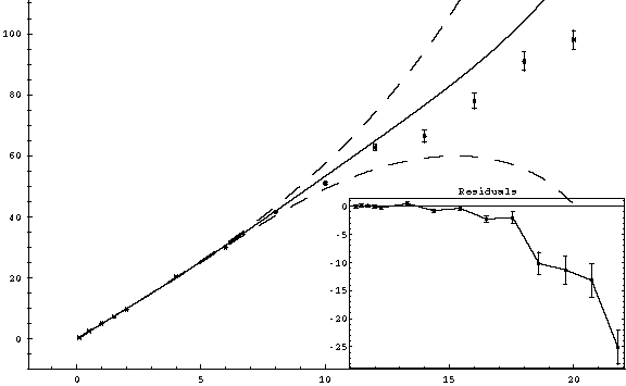
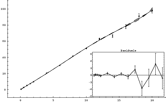
This is actually worse than the 4th order fit!! The residuals have increased, and the curve deviates away from the data. This fit is WRONG!! The value of χ2 which it reports is also wrong. You can tell from the residuals that χ2 must be a few hundred at least. The problem is that by default the faraday fitter requires that the fitted parameters have the same number of significant figures as the input data. So, since the exact value of some of the coefficients is important for the higher order polynomials, rounding error throws off the fit. The way to fix it is to click on Advanced Options and select False for UseSignificantFigures. It is probably best to set this option to false for ALL fits. The 6th order polynomial now looks like:

which is much MUCH
better! Now, in fact, we have “over-fit”
these particular data, and the linear fit is in fact much more appropriate in
this case. But I have given this as an
example so that you might be careful with the UseSignificantFigures option.
Back to Faraday Hints.